Spatiotemporal analysis of synthetic data
This notebook gives some examples of spatiotemporal analysis that we can conduct using eggplant’s framework. To demonstrate this we generate some synthetic data and then analyze it. In large it encompasses four main steps:
Generation of time series data using a dynamical system based on ODEs
Generation of spatial synthetic data based on time series data
Transfer of data to a common reference
Estimation of system parameters from transferred data
Import libraries
[1]:
import numpy as np
import matplotlib.pyplot as plt
from matplotlib import rcParams
from scipy.integrate import odeint
from PIL import Image


import anndata as ad
import pandas as pd
import sys
import os.path as osp


import eggplant as eg

from eggplant import ode
[16]:
SAVE_MODE = False
1. Generation of time series data using a dynamical system based on ODEs
Configure figure settings
[3]:
rcParams["figure.facecolor"] = "none"
rcParams["axes.facecolor"] = "none"
set random seed, for reproducibility
[4]:
np.random.seed(27)
Define model parameters, according to: \begin{equation} \begin{bmatrix} r_{11} & r_{12}\\ r_{21} & r_{22} \end{bmatrix} \end{equation}
[5]:
n_regions = 2
rs = np.array([[0.2,0.8],[0.1,-0.3]])
rs
[5]:
array([[ 0.2,  0.8],
       [ 0.1, -0.3]])
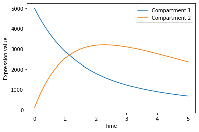
set initial values \(\boldsymbol{x}(0) = (x_1(0),x_2(0)) = (5000,100)\)
[6]:
x0 = np.array([5000,100])
- Define model dynamics, according to: :nbsphinx-math:`begin{equation}
begin{array}{l} frac{dc_{1}}{dt} = (r_{11}-r_{12})c_1 + r_{21}c_2\[4pt]
- frac{dc_{2}}{dt} = (r_{22}-r_{21})c_2 + r_{12}c_1\
end{array} label{eq:dynamics}
end{equation}` and propagate in time, i.e., solving the system over the time points \(\mathcal{T} = \{t : t \in [0,1000], t \textrm{ mod } 5 = 0\}\).
[7]:
ode_fun = ode.make_ode_fun(n_regions = 2)
time = np.linspace(0,5,1000)
soln = odeint(ode_fun,x0,time,args = (rs,))
Visualize system over time
[8]:
plt.plot(time,
         soln[:,0],
         label = "Compartment 1",
        )
plt.plot(time,
         soln[:,1],
         label = "Compartment 2",
        )

plt.ylabel("Expression value")
plt.xlabel("Time")
plt.legend()
plt.show()
Check that the ODE solver works when presented with full data; this is more a check of the solver implementation than anything else.
[9]:
odeS = ode.ODE_solver(time,
                      soln,
                      x0,
                      ode_fun,
                      )

prms = odeS.optim(np.zeros(n_regions*n_regions))
We reshape the inferred parameters (solver does not work with 2d arrays) and then compare it with the true parameter values
[10]:
rs_pred = prms["x"].reshape(n_regions,n_regions)
[11]:
vmin = min(rs_pred.min(),rs.min())
vmax = max(rs_pred.max(),rs.max())
plt.subplot(121)
im1 = plt.imshow(rs,vmin = vmin,vmax = vmax,cmap = plt.cm.magma)
plt.colorbar(im1,)
plt.axis("equal")
plt.axis("off")
plt.title("True")
plt.subplot(122)
im2 = plt.imshow(rs_pred,vmin = vmin,vmax = vmax,cmap = plt.cm.magma)
plt.colorbar(im2)
plt.axis("equal")
plt.axis("off")
plt.title("Estimated")
plt.show()
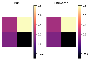
Everything looks good, and we can proceed to construct the synthetic data
2. Generation of spatial synthetic data based on time series data
We define the paths to the templates used for the synthetic data and their landmark annotations.
[12]:
SYN_DIR = "../../../data/synthetic/"
img_paths = [osp.join(SYN_DIR,"templates","imgs","t_{}.png".format(x)) for x in range(0,8)]
lmk_paths = [osp.join(SYN_DIR,"templates","landmarks","t_{}_landmarks.tsv".format(x)) for x in range(0,8)]
We next load each template and its corresponding landmark annotations. Each template is assigned to one time points and we distribute the number of transcripts between each compartment according to the system dynamics. Since we are using two compartments (marked in different colors in the reference), we set n_regions=2, we will again use approximately 1000 points in our reference grid.
[13]:
from PIL import Image
sel_times = np.linspace(0,int(len(time) / 2),8).round().astype(int)
new_int_soln = soln
crds = list()
counts = list()
lmks = list()
for ii,(img_pth,lmk_pth,t) in enumerate(zip(img_paths,
                                            lmk_paths,sel_times)):
    lmk = pd.read_csv(lmk_pth,
                      sep = "\t",
                      header = 0,
                      index_col = 0)
    lmks.append(lmk)
    img = Image.open(img_pth)
    crd,meta = eg.pp.reference_to_grid(img,
                                      n_approx_points=1000,
                                      background_color="white",
                                      n_regions=2,
                                      )

    count = np.zeros(crd.shape[0])

    for k,reg in enumerate(np.unique(meta)):
        idx = np.where(meta == reg)[0]
        size = int(new_int_soln[t,k])
        sel = np.random.choice(idx,
                               replace = True,
                               size = size)
        for s in sel:
            count[s] +=1

    crds.append(crd)
    counts.append(count)
Next, we convert the count matrices and landmark data into AnnData objects that are easy to operate with and compatible with the eggplant API.
[14]:
adatas = []
for k in range(len(crds)):
    obs_index = [f"Spot_{x}" for x in range(len(crds[k]))]
    adata = ad.AnnData(counts[k][:,np.newaxis],
                       var = pd.DataFrame(["Gene1"],
                                          columns = ["Gene"],
                                          index = ["Gene1"],
                                         ),
                       obs = pd.DataFrame(index = obs_index)
                      )
    adata.obsm["spatial"] = crds[k]
    adata.uns["curated_landmarks"] = lmks[k]
    eg.pp.get_landmark_distance(adata)
    adatas.append(adata)
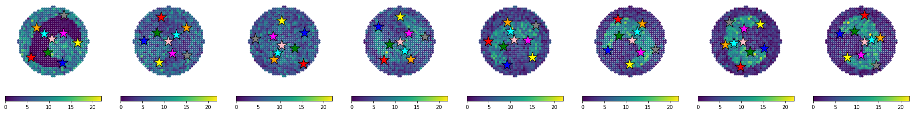
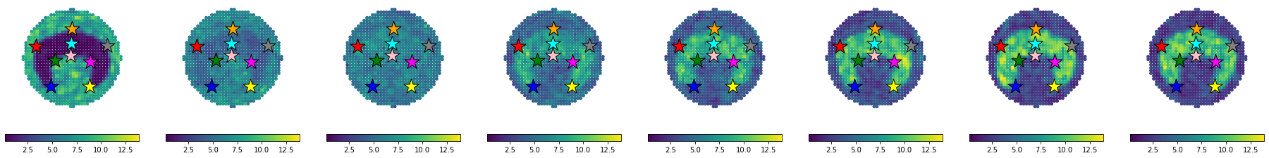
We visualize the generated data to check that everything is in order. The visualization below is the raw images used to assemble Figure 1B in the manuscript, hence why the colorbar is in a seprate figure and no titles are included.
[18]:
eg.pl.visualize_observed(adatas,
                         features="Gene1",
                         quantile_scaling = False,
                         n_rows = 1,
                         separate_colorbar = False,
                         include_title = False,
                         marker_size = 15,
                         colorbar_fontsize = 10,
                        )
3. Transfer of data to a common reference
We begin the transfer by reading in the reference template and its associated landmarks
[19]:
ref_lmk_pth = osp.join(SYN_DIR,"references","landmarks.tsv")
ref_img_pth = osp.join(SYN_DIR,"references","reference.png")
ref_lmk = pd.read_csv(ref_lmk_pth,sep = "\t",header = 0,index_col = 0)
ref_img = Image.open(ref_img_pth)
ref_crd,ref_meta = eg.pp.reference_to_grid(ref_img,
                                           n_approx_points=1000,
                                           background_color="white",
                                           n_regions=2,
                                          )
Next we assemble a Reference object from the reference array data and landmarks. We also mathc the distances between our observed data and the reference, as well as compute landmark distances after correcting for non-homogenous distortions.
[20]:
ref_lmk
[20]:
| x_coord | y_coord | |
|---|---|---|
| Landmark_0 | 412.176 | 663.138 |
| Landmark_1 | 109.692 | 513.558 |
| Landmark_2 | 234.342 | 174.510 |
| Landmark_3 | 268.413 | 394.725 |
| Landmark_4 | 404.697 | 438.768 |
| Landmark_5 | 570.897 | 383.922 |
| Landmark_6 | 564.249 | 174.510 |
| Landmark_7 | 716.322 | 520.206 |
| Landmark_8 | 405.528 | 541.812 |
[21]:
ref = eg.m.Reference(ref_crd,
                     landmarks = ref_lmk,
                    )

for adata in adatas:
    eg.pp.match_scales(adata,ref)
    eg.pp.get_landmark_distance(adata,
                                reference=ref)
Finally, we can conduct the transfer from the observed data to the reference
[22]:
!export CUDA_VISIBLE_DEVICES=0
[23]:
losses = eg.fun.transfer_to_reference(adatas,
                                      "Gene1",
                                      ref,
                                      device = "gpu",
                                      n_epochs=1000,
                                      verbose = True,
                                      return_models =False,
                                      return_losses = True,
                                      )
[Processing] :: Model : Model_0 | Feature : Gene1 | Transfer : 1/8
/home/alma.andersson/miniconda3/envs/eggplant2/lib/python3.8/site-packages/eggplant-0.1-py3.8.egg/eggplant/models.py:69: UserWarning: To copy construct from a tensor, it is recommended to use sourceTensor.clone().detach() or sourceTensor.clone().detach().requires_grad_(True), rather than torch.tensor(sourceTensor).
  self.ldists = t.tensor(landmark_distances)
/home/alma.andersson/miniconda3/envs/eggplant2/lib/python3.8/site-packages/eggplant-0.1-py3.8.egg/eggplant/models.py:70: UserWarning: To copy construct from a tensor, it is recommended to use sourceTensor.clone().detach() or sourceTensor.clone().detach().requires_grad_(True), rather than torch.tensor(sourceTensor).
  self.features = t.tensor(feature_values)
  0%|                                                                                                                         | 0/1000 [00:00<?, ?it/s]/home/alma.andersson/miniconda3/envs/eggplant2/lib/python3.8/site-packages/gpytorch/utils/linear_cg.py:266: UserWarning: An output with one or more elements was resized since it had shape [11], which does not match the required output shape [1, 11].This behavior is deprecated, and in a future PyTorch release outputs will not be resized unless they have zero elements. You can explicitly reuse an out tensor t by resizing it, inplace, to zero elements with t.resize_(0). (Triggered internally at  ../aten/src/ATen/native/Resize.cpp:23.)
  _jit_linear_cg_updates_no_precond(
100%|██████████████████████████████████████████████████████████████████████████████████████████████████████████████| 1000/1000 [00:23<00:00, 42.54it/s]
[Processing] :: Model : Model_1 | Feature : Gene1 | Transfer : 2/8
/home/alma.andersson/miniconda3/envs/eggplant2/lib/python3.8/site-packages/anndata/_core/anndata.py:120: ImplicitModificationWarning: Transforming to str index.
  warnings.warn("Transforming to str index.", ImplicitModificationWarning)
100%|██████████████████████████████████████████████████████████████████████████████████████████████████████████████| 1000/1000 [00:23<00:00, 42.96it/s]
[Processing] :: Model : Model_2 | Feature : Gene1 | Transfer : 3/8
100%|██████████████████████████████████████████████████████████████████████████████████████████████████████████████| 1000/1000 [00:22<00:00, 44.66it/s]
[Processing] :: Model : Model_3 | Feature : Gene1 | Transfer : 4/8
100%|██████████████████████████████████████████████████████████████████████████████████████████████████████████████| 1000/1000 [00:25<00:00, 39.77it/s]
[Processing] :: Model : Model_4 | Feature : Gene1 | Transfer : 5/8
100%|██████████████████████████████████████████████████████████████████████████████████████████████████████████████| 1000/1000 [00:23<00:00, 42.04it/s]
[Processing] :: Model : Model_5 | Feature : Gene1 | Transfer : 6/8
100%|██████████████████████████████████████████████████████████████████████████████████████████████████████████████| 1000/1000 [00:23<00:00, 41.67it/s]
[Processing] :: Model : Model_6 | Feature : Gene1 | Transfer : 7/8
100%|██████████████████████████████████████████████████████████████████████████████████████████████████████████████| 1000/1000 [00:23<00:00, 42.41it/s]
[Processing] :: Model : Model_7 | Feature : Gene1 | Transfer : 8/8
100%|██████████████████████████████████████████████████████████████████████████████████████████████████████████████| 1000/1000 [00:23<00:00, 42.88it/s]
Let us check the loss curves to make sure that the models converge and that nothing unexpected happened.
[24]:
eg.pl.model_diagnostics(losses = losses)
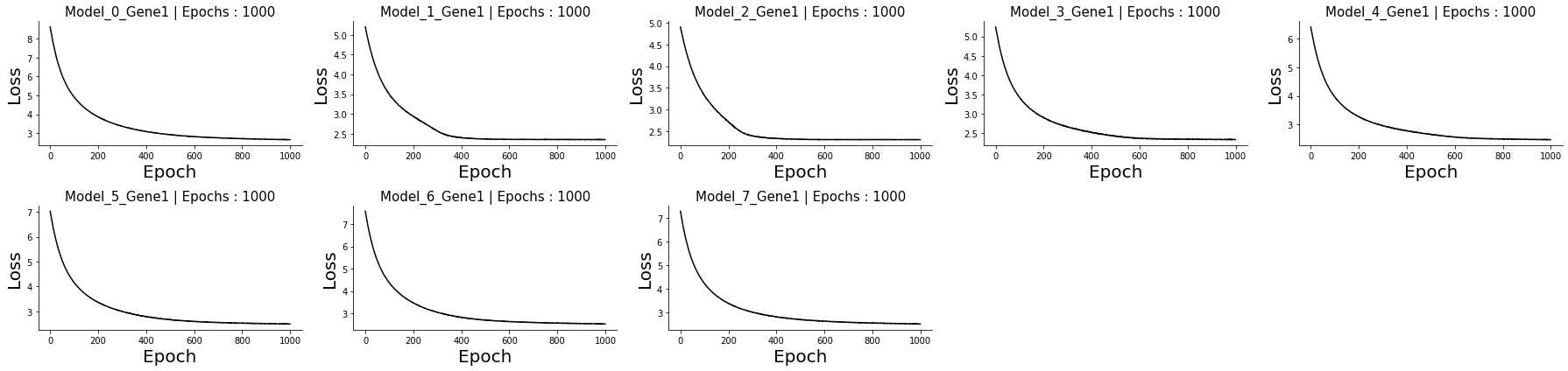
Since everything looks as expected, we proceed to visualize the results spatially.
[26]:
eg.pl.visualize_transfer(ref,
                         marker_size = 15,
                         separate_colorbar=False,
                         n_rows = 1,
                         include_title =False,
                         colorbar_fontsize = 10,
                        )
4. Estimation of system parameters from transferred data
Parameter estimation
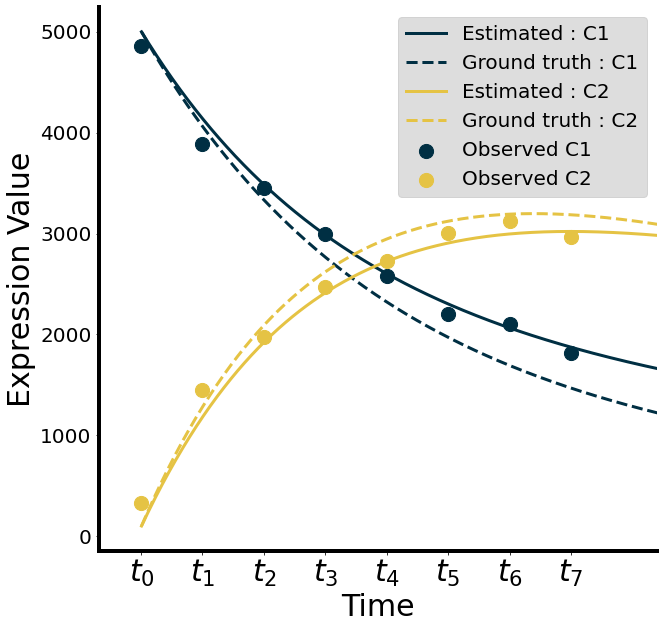
In the spatiotemporal analysis we try to infer the rate parameters \((r_{11},r_{12},r_{21},r_{22})\) from the transferred data. Since we know the character of the systems dynamics, this becomes a task of fitting a model to the data. However, the very fist thing we need to do is to aggregate the expected number of transcripts in each compartment (C1 and C2), which we do below.
[28]:
time_data = np.zeros((len(adatas),n_regions))

for t in range(len(adatas)):
    for k,reg in enumerate([0,1]):
        idx = ref_meta == reg
        time_data[t,k] = np.sum(ref.adata.X[idx,t])
Next we apply the ODE solver using out aggregated data and the time points at which we sampled it from.
[29]:
odes = ode.ODE_solver(time[sel_times],
                  time_data,
                  time_data[0,:],
                    ode_fun=ode_fun,
                  )

prms = odes.optim(np.zeros(n_regions*n_regions))
We then continue to solve the system using the estimated parameters
[30]:
est_rs = prms["x"].reshape(n_regions,n_regions)
est_soln = odeint(ode_fun,
                  x0,
                  time,
                  args = (est_rs,),
                 )
Now we compare the true and estimated solution to see how well our estimates performed.
[31]:
# Output used for Figure 2C
fig,ax = plt.subplots(1,1,figsize=(10,10))
for k,(clr,compname) in enumerate(zip(["#002F43","#E5C344"],
                             ["C1","C2"])):

    ax.scatter(sel_times,
           time_data[:,k],
           c = clr,
           s = 200,
           label = "Observed " + compname,
           )

    for sol,linetype,solname in zip([est_soln,soln],
                                    ["solid","dashed"],
                                    ["Estimated","Ground truth"]):

        ax.plot(sol[:,k],
                color = clr,
                linestyle = linetype,
                label = solname + " : " + compname,
                linewidth = 3,
               )

ax.set_xticks(sel_times)
ax.set_xticklabels([r"$t_{}$".format(k) for k in range(len(sel_times))],
                 fontsize = 30.
                 )

plt.setp(ax.get_yticklabels(), fontsize=20)

ax.legend(fontsize = 20, facecolor ="#D5D5D5")
ax.set_ylabel("Expression Value",fontsize = 30)
ax.set_xlabel("Time",fontsize = 30)
[i.set_linewidth(4) for i in ax.spines.values()]
ax.spines["top"].set_visible(False)
ax.spines["right"].set_visible(False)
ax.set_xlim([-50,600])

if SAVE_MODE: plt.savefig(osp.join(RES_DIR,"synthetic-1-system.png"))
plt.show()
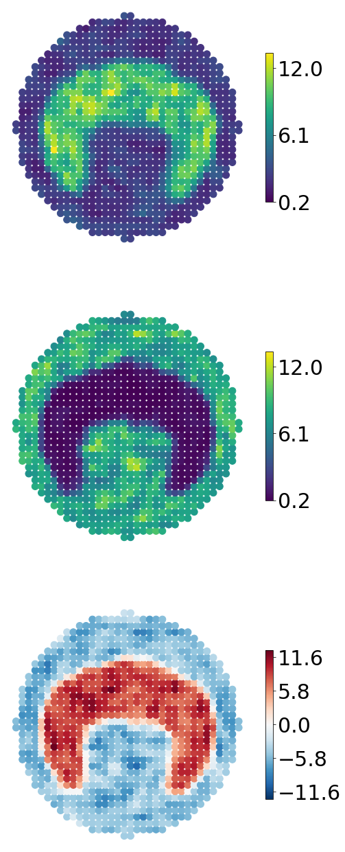
Spatial Arithmetics
Our final analysis will be swift and simple, yet effectful. We will conduct what is here referred to as spatial arithmetics. More precisely this procedure allows us to highlight local difference between time points or conditions in the feature that we’ve mapped to our reference; in our case this will evidently be over time points In practice, since our data have been transferred to the same reference we can simply subtract the values of one location at \(t_1\) from the values at the very same location at \(t_2\), and we’ll be able to see how the feature of interest differs in this region between the two time points. If we do this for every point in the reference array, we’ll end up with a map of local changes, providing a global overview. We’ll look at the local changes between the first and lost time point here.
[32]:
# Output used in Figure 1D
fig,ax = plt.subplots(3,1,figsize = (8,24))
ax = ax.flatten()
art_sel = [-1,0]
vmin = ref.adata.X[:,art_sel].min()
vmax = ref.adata.X[:,art_sel].max()
cticks = np.linspace(vmin * 1.1,vmax * 0.9,3).round(1)

marker_size = 100
cbar_fontsize = 30
art_cmaps = [plt.cm.Reds,plt.cm.Blues]

for k,s in enumerate(art_sel):
    _sc = ax[k].scatter(ref_crd[:,0],
                        ref_crd[:,1],
                        c = ref.adata.X[:,s],
                        s = marker_size,
                        cmap = plt.cm.viridis,
                        marker = "o",
                        vmin = vmin,
                        vmax = vmax,
                       )

    cbar = fig.colorbar(_sc,ax = ax[k],shrink = 0.5,ticks=cticks)
    cbar.ax.tick_params(labelsize=cbar_fontsize)


diff = ref.adata.X[:,[art_sel[0]]] - ref.adata.X[:,[art_sel[1]]]
vmin = diff.min()
vmax = diff.max()

vmax = max(abs(vmin),abs(vmax))
vmin = -vmax

cticks= np.linspace(vmin + abs(0.1*vmax),vmax - 0.1*abs(vmax),5).round(1)

_sc = ax[2].scatter(ref_crd[:,0],
              ref_crd[:,1],
              c = diff ,
              s = marker_size,
              cmap = plt.cm.RdBu_r,
              marker = "o",
              vmin = vmin,
              vmax = vmax,
             )

cbar = fig.colorbar(_sc,
                    ax = ax[2],
                    shrink=0.5,
                    ticks=cticks)

cbar.ax.tick_params(labelsize=cbar_fontsize,)


for aa in ax:
    aa.set_aspect("equal")
    aa.axis("off")


plt.subplots_adjust(hspace = 0.0001)
plt.show()